The Hopf invariant (in particular) is a homotopy invariant of map between spheres:
(1.1) i.e. continuous mapping from the unit 3-sphere (wiki) to the ordinary sphere with unit radius [H.Hopf "Über die Abbildungen der dreidimensionalen Sphäre auf die Kugelfläche", Math. Annalen 104 (1931), 637 ref]. The 3-sphere is a four-dimensional object and it is difficult to imagine. But what's important. The usual stereographic projection (wiki) correlates all points of the plane including infinity with the usual sphere. Вy analogy, there is a correlation between all points from the real space (including infinity) and 3-sphere:
(1.2)
i.e. continuous mapping from the unit 3-sphere (wiki) to the ordinary sphere with unit radius [H.Hopf "Über die Abbildungen der dreidimensionalen Sphäre auf die Kugelfläche", Math. Annalen 104 (1931), 637 ref]. The 3-sphere is a four-dimensional object and it is difficult to imagine. But what's important. The usual stereographic projection (wiki) correlates all points of the plane including infinity with the usual sphere. Вy analogy, there is a correlation between all points from the real space (including infinity) and 3-sphere:
(1.2) This allows us to write the map (1.1) in a more understandable form
(1.3)
This allows us to write the map (1.1) in a more understandable form
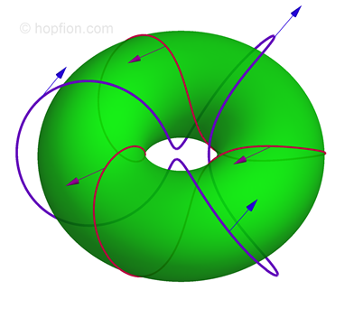
(1.3) Thus, each point of the real space mapped to a point on the ordinary sphere, but infinite points are mapped in one specific point on the sphere. An example of such a map is any continuous uniform 3D vector field homogeneous at infinity. Image in this case is the point on the unit sphere - that is, direction of the vector. The preimage is a some curve in real space. Important property is that set of homotopy classes of such maps is an isomorphism with integers:
(1.4)
Thus, each point of the real space mapped to a point on the ordinary sphere, but infinite points are mapped in one specific point on the sphere. An example of such a map is any continuous uniform 3D vector field homogeneous at infinity. Image in this case is the point on the unit sphere - that is, direction of the vector. The preimage is a some curve in real space. Important property is that set of homotopy classes of such maps is an isomorphism with integers:
(1.4) In fact, this difficult expression means the following. If we have a continuous unit vector field homogeneous at infinity, we can calculate a some number corresponding to this field. This number is necessarily an integer. If we make a smooth deformation, then the number will remain the same. In addition, this number is a unique characteristic, which means that all sorts of different configurations with the same numbers can be transformed into each other by a continuously deformation. This "magic number" is called Hopf index and can be calculated for any smooth unit vector field
(1.5)
In fact, this difficult expression means the following. If we have a continuous unit vector field homogeneous at infinity, we can calculate a some number corresponding to this field. This number is necessarily an integer. If we make a smooth deformation, then the number will remain the same. In addition, this number is a unique characteristic, which means that all sorts of different configurations with the same numbers can be transformed into each other by a continuously deformation. This "magic number" is called Hopf index and can be calculated for any smooth unit vector field
(1.5) For the first time the direct formula was found by Whitehead [J.H.C. Whitehead "An expression of Hopf’s invariant as an integral", Proc. Nat. Acad. Sci. U.S.A. 33 (1947), 117 ref] and expression for Hopf index can be written as
(1.6)
For the first time the direct formula was found by Whitehead [J.H.C. Whitehead "An expression of Hopf’s invariant as an integral", Proc. Nat. Acad. Sci. U.S.A. 33 (1947), 117 ref] and expression for Hopf index can be written as
(1.6)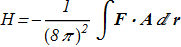 where two additional vector fields are defined explicitly and implicitly
(1.7)
where two additional vector fields are defined explicitly and implicitly
(1.7)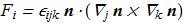 (1.8)
(1.8)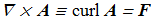 where Levi-Civita symbol and gradient operator are used, summations over the indices are assuming. In case of natural parameterization by angles
(1.9)
where Levi-Civita symbol and gradient operator are used, summations over the indices are assuming. In case of natural parameterization by angles
(1.9) the F definition is simpler:
(1.10)
the F definition is simpler:
(1.10)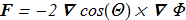
Here is a concrete example for the calculation of the index for symmetric Hopf fibration. Let
(1.11) in cylindrical coordinate system (ρ,φ,z). Then there is a solution for vector potential [J. Gladikowski, M. Hellmund "Static solitons with non-zero Hopf number", arXiv:hep-th/9609035v1; Phys. Rev. D 56, 5194 (1997) ref] which satisfies the equation (1.8):
(1.12)
in cylindrical coordinate system (ρ,φ,z). Then there is a solution for vector potential [J. Gladikowski, M. Hellmund "Static solitons with non-zero Hopf number", arXiv:hep-th/9609035v1; Phys. Rev. D 56, 5194 (1997) ref] which satisfies the equation (1.8):
(1.12)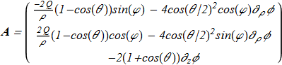 Direct verification shows that
(1.13)
Direct verification shows that
(1.13)
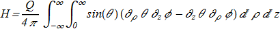 Thus we get Q-times multiplied topological charge of the
  type vortex which lies in a half-plane (ρ,z).
* There is also an indirect way to determine the Hopf index for a given field - the linking number (wiki) of preimages.